Let's say we have an STFT with some sampling frequency fs and a frame size nf, this implies a frequency range of fs / 2 (Nyquist frequency) and a resolution of res = fs / nf.

This leads to an output where each frequency index fi represents the frequency at fi * res.

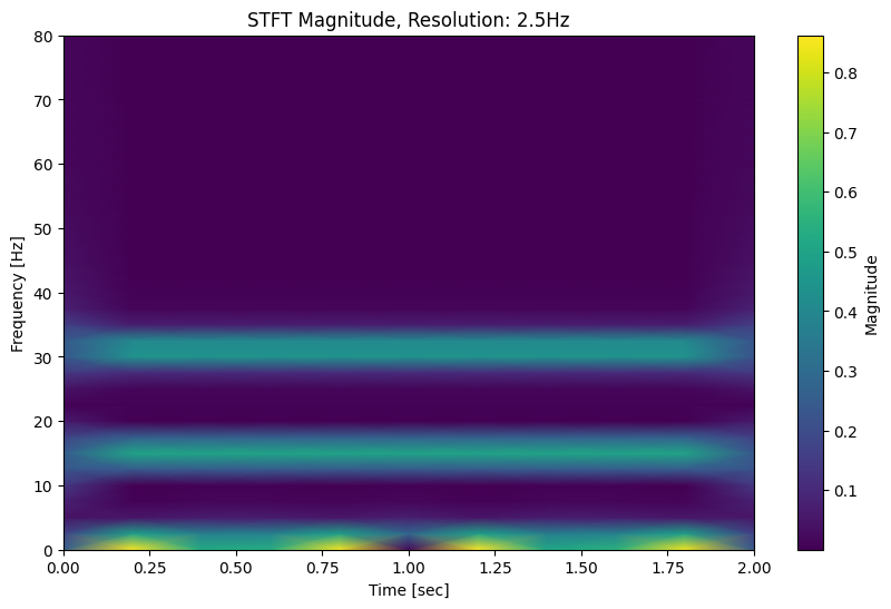
As an example, a fs of 160 and nf = 64, we get a resolution of ~2.5Hz.

Are target frequencies then handled differently if they land perfectly on a multiple of the resolution?

To answer that, I'll have to generate a wave with frequencies e.g. 1Hz, 3Hz and 5Hz and see what vaues two different frame lengths give us, one providing a resolution of 2.5Hz, and the other a resolution of 1Hz

import numpy as np
import matplotlib.pyplot as plt
from scipy.signal import stft

fs = 160
t = 2
x = (np.linspace(0, 1, t * fs)) * t * 2 * np.pi
print(x.shape)
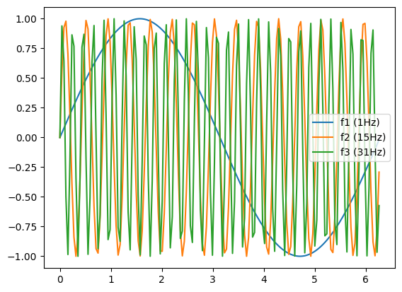
f1 = np.sin(x)
f2 = np.sin(15 * x)
f3 = np.sin(31 * x)

# Just display the first second 
plt.plot(x[:fs], f1[:fs], label='f1 (1Hz)')
plt.plot(x[:fs], f2[:fs], label='f2 (15Hz)')
plt.plot(x[:fs], f3[:fs], label='f3 (31Hz)')
plt.legend()
plt.show()

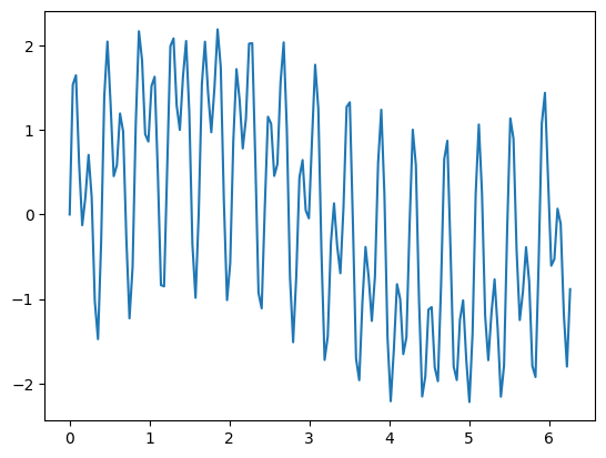
fc = f1 + f2 + f3
plt.plot(x[:fs], fc[:fs], label='Combined')
plt.show()

(320,)

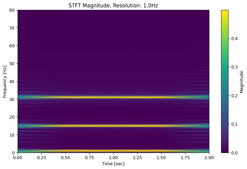
for nf in [160, 64]:
    print(f"resolution: {fs / nf}Hz")
    rect = np.ones(nf) # remove windowing to prevent leakage due to windowing
    f, t, Zxx = stft(fc, fs=fs, window=rect, nperseg=nf, noverlap=nf / 2)
    
    # Plot the STFT Magnitude
    plt.figure(figsize=(10, 6))
    plt.pcolormesh(t, f, np.abs(Zxx), shading='gouraud')
    plt.title(f'STFT Magnitude, Resolution: {fs / nf}Hz')
    plt.ylabel('Frequency [Hz]')
    plt.xlabel('Time [sec]')
    plt.colorbar(label='Magnitude')
    plt.show()

resolution: 1.0Hz

resolution: 2.5Hz

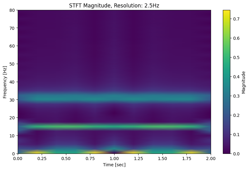
So we can see from this example that yes, the total energy in the spectrogram is spread out differently depending on whether the underlying frequency lands on the resolution boundary.

The reason for this is the same as the problem of spectral leakage caused by very low frequencies or drifting. Even though the "full-resolution" version has all 80 frequencies as its analysis frequencies, the lower-resolution version does not. Applying windowing shows this effect:

nf = 64
print(f"resolution: {fs / nf}Hz")
f, t, Zxx = stft(fc, fs=fs, window='hann', nperseg=nf, noverlap=nf / 2)

# Plot the STFT Magnitude
plt.figure(figsize=(10, 6))
plt.pcolormesh(t, f, np.abs(Zxx), shading='gouraud')
plt.title(f'STFT Magnitude, Resolution: {fs / nf}Hz')
plt.ylabel('Frequency [Hz]')
plt.xlabel('Time [sec]')
plt.colorbar(label='Magnitude')
plt.show()

resolution: 2.5Hz

And now we see the frequency energy spread out, but handled equally (except that the 1Hz frequency looks pretty funky at the edge there... not sure why that is).

Finally, since we intend to take quantiles over frequency bins, all that I'm really concerned about is that the full frequency energy is captured per frequency bin, even if it gets spread out in the lower-resolution stft.

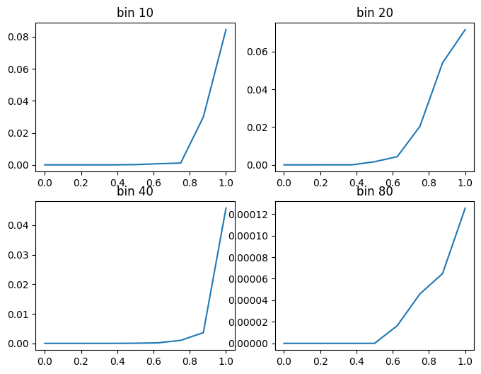
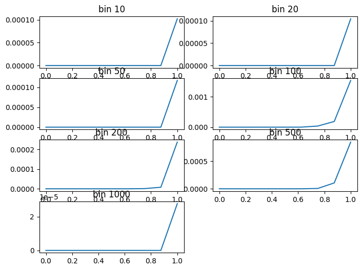
f_bins = [10, 20, 40, 80]
p: np.ndarray = np.arange(9) * 10 + 10

for nf in [160, 64]:
    print(f"resolution: {fs / nf}Hz")
    rect = np.ones(nf) # remove windowing to prevent leakage due to windowing
    f, t, Zxx = stft(fc, fs=fs, window='hann', nperseg=nf, noverlap=nf / 2)

    X = np.abs(Zxx) ** 2
    fp = 0
    out = []
    for i in f_bins:
        out.append(np.percentile(X[(fp <= f) & (f < i), :].flatten(), p).tolist())
        fp = i

    plt.figure(figsize=(8, 6))  # Optional: set figure size
    for i, cdf in enumerate(out):
        x = np.linspace(0, 1, len(p))
        plt.subplot(2, 2, i + 1)  # (rows, columns, plot number)
        plt.plot(x, np.array(cdf))
        plt.title(label=f'bin {f_bins[i]}')
    plt.show()

resolution: 1.0Hz

resolution: 2.5Hz

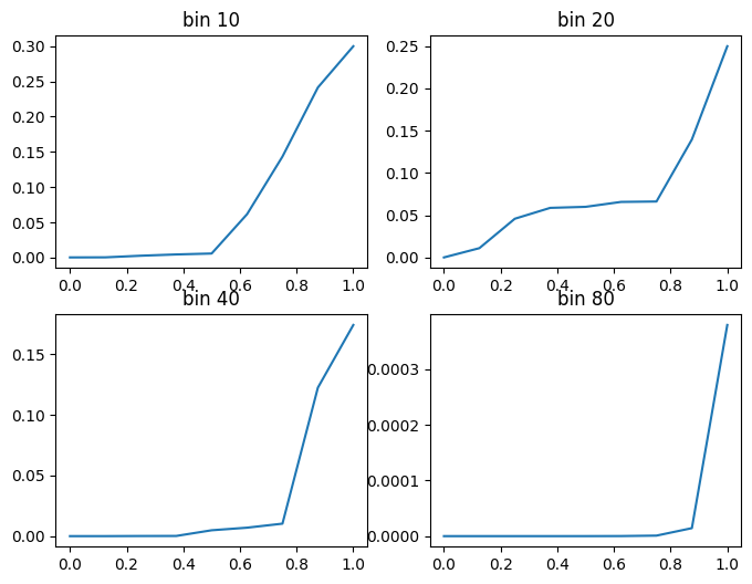
Okay, so the lower resolution indeed affects the quantiles of the frequency bins. This actually makes sense, as the lower resolution reduces the sharpness of the detected frequencies, which is another way of saying that the distribution becomes flatter!

However, all hope is not lost, as this effect is probably rather pronounced for low frequency bins, where the resolution is on the same order of magnitude as the bin size. But what about when dealing with kHz over a resolution of 2.5Hz?

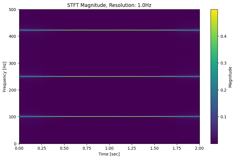
Let's repeat the experiment with larger frequencies

fs = 1000
t = 2
x = (np.linspace(0, 1, t * fs)) * t * 2 * np.pi
print(x.shape)
f1 = np.sin(101 * x)
f2 = np.sin(250 * x)
f3 = np.sin(577 * x) #A prime number, just to be tricky

fc = f1 + f2 + f3

f_bins = [10, 20, 50, 100, 200, 500, 1000]
p: np.ndarray = np.arange(9) * 10 + 10

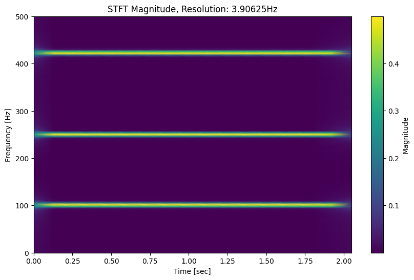
for nf in [1000, 256]:
    print(f"resolution: {fs / nf}Hz")
    #rect = np.ones(nf) # remove windowing to prevent leakage due to windowing
    f, t, Zxx = stft(fc, fs=fs, window='hann', nperseg=nf, noverlap=nf / 2)
    
    # Plot the STFT Magnitude
    plt.figure(figsize=(10, 6))
    plt.pcolormesh(t, f, np.abs(Zxx), shading='gouraud')
    plt.title(f'STFT Magnitude, Resolution: {fs / nf}Hz')
    plt.ylabel('Frequency [Hz]')
    plt.xlabel('Time [sec]')
    plt.colorbar(label='Magnitude')
    plt.show()

    X = np.abs(Zxx) ** 2
    fp = 0
    out = []
    for i in f_bins:
        out.append(np.percentile(X[(fp <= f) & (f < i), :].flatten(), p).tolist())
        fp = i

    plt.figure(figsize=(8, 6))  # Optional: set figure size
    for i, cdf in enumerate(out):
        x = np.linspace(0, 1, len(p))
        plt.subplot(4, 2, i + 1)  # (rows, columns, plot number)
        plt.plot(x, np.array(cdf))
        plt.title(label=f'bin {f_bins[i]}')
    plt.show()

(2000,)
resolution: 1.0Hz

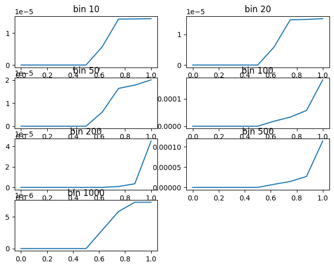
resolution: 3.90625Hz

Hmm, it looks like the quantiles are still pretty sensitive to the difference. This is unexpected. I'll have to look deeper here.